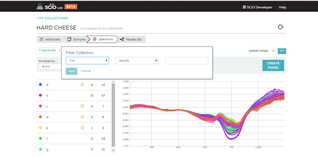
Data Collections are the grouping of similar sample materials, their corresponding scans and meta data. Your scans are stored in both SCiO Lab and in SCiO Lab mobile in the data collections you create for them. Your SCiO Lab account comes with two default data collections. Start Here and Hard Cheese. Hard Cheese is included to serve as an example of how a well formed data collection should look. Start Here is an empty collection for you to use to get started from.

More information about how to work with data collections is available here and here.

Models are the mathematical means of transforming your scan spectra into data. Your models are created directly from your data collections which is why well formed data collections are so critical to the ultimate success of your models. Models can be either estimation or classification based. More information about Models and Model Types is available here and here.

SCiO occasionally requires re-calibration in order to create accurate readings for every sample. The SCiO Cover comes with a built in calibration tool for your SCiO. SCiO Lab Mobile knows when your SCiO requires calibration and will notify you on screen when calibration is required. Instructions about how to calibrate your SCiO can be found here.

Scanning small samples


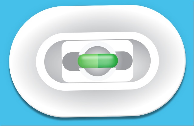
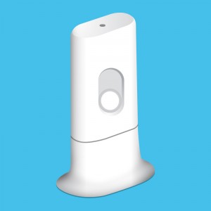
The Solid Sample Holder is a scanning accessory to use when your sample is too small to fill the entire illumination field (such as with a pill or a capsule).

pill-accessory
Solid Sample Holder


To use the Solid Sample Holder correctly:
  1. Place SCiO in the cover, with the optical head facing out.
  2. Place the solid, dry sample into the sample holder and center it into the scan field.
    pill_in_middle
  3. Place the SCiO on top of the sample holder with the optical head facing the scan field. Magnets within the sample holder and SCiO will hold it in place.
    stacked
  4. Release your hand from holding SCiO on the sample holder (it will stay with the magnets) and tap scan on your phone.
  5. Once you see the scan is finished, remove SCiO from on top of the sample holder and repeat for your next scan.
Important note: The Solid Sample Holder cannot be used for liquids or semi-solids of any type. Only samples small enough to fit easily and that are completely dry should be placed in the holder. Scratching the internal coating of the holder, or getting it wet,  will both void your warranty and destroy the holder.

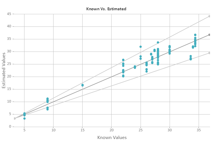
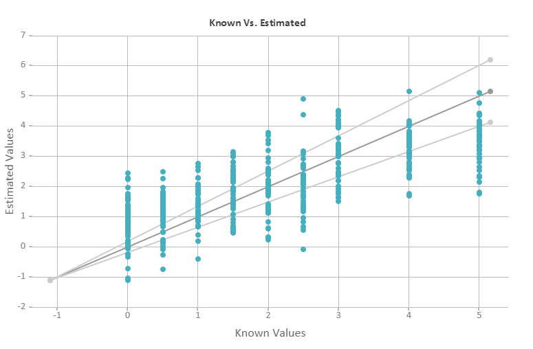
When you assess the performance of an estimation model you’ll want to use the Known vs. Estimated scatter plot.

In an ideal situation your model estimated value is the same as the known value. But the reality is that noise and other effects can influence your results and this does not occur. To analyze the success or failure of your potential model, SCiO Lab enables you to view the results as a scatter plot.

To create a scatter plot:

    1. Navigate to the Spectrum tab of a Data Collection
    2. Select an attribute to filter the model building from using the Analyze by filter on the left side of the screen.

      1. Apply one of the pre-designed preprocessing methods or create your own using the expert mode.
      2. Click Create Model.
      3. Your model’s performance is displayed as a Known vs. Estimated Scatter Plot, and provides performance metrics and if needed, suggestions for improvement. If you model does not contain enough samples, a warning will appear above your Scatter Plot, alerting you to scan more before trying to build.


Good Model_known vs estimated

Good Scatter Plot

Bad Model_known vs estimated

Bad scatter plot

On each scatter plot, the horizontal axis shows the known values and the vertical axis displays the estimated values. Each point on the scatter plot represents a data point (one scan). In the scatter plot, the central line represents the optimal model. The upper and lower limit lines represent the 20% error margin.

SCiO’s estimation algorithms assume a linear dependency between sample attributes and the algorithmic inputs. However, SCiO measures the reflection spectra, which does not have that linear dependence but is rather exponential, according to the Beer-Lambert model.
Our “processed” algorithm transforms the scanned spectra to a form that is linear with concentration by performing a log transform and taking the first derivative (with respect to wavelength) and removing the average. Removing the average of the results helps to correct discrepancies from the Beer-Lambert model.


Note: The Beer-Lambert model removes gain, but SNV is better at it.

Processing takes the log (natural algorithm), then the first derivative and then removes the average. It removes gain, but more importantly , transforms the equation to be linear with concentration (assuming the Beer-Lambert model applies).

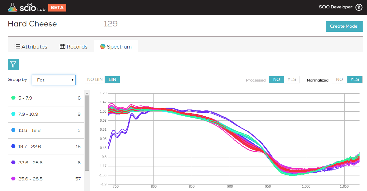
Normalization removes the average and divides by the standard deviation. When normalization is applied in conjunction with processed, it compensates for optical path differences. When used alone, it compensates for gain.

For example, compensation is applied for the possible distance irregularities that are likely to occur when scanning different samples. SCiO’s normalized spectrum apply the industry standard calculation of SNV.

For more information about SNV deviation, see here:  Advanced Preprocessing: Sample Normalization

Normalized_Results - Copy

Normalized, No Processing

Normalized_not

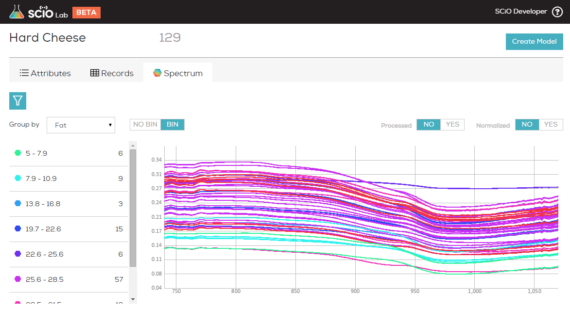
Not Notmalized, Not Processed (Raw Reflectance)