PCA stands for Principle Component Analysis. It is a common tool in machine learning in general, and even more in chemometrics. PCA is a technique used to emphasize variation and bring out strong patterns in the spectra (read more about it here). In SCiO Lab, PCA is used to make data easier to explore and visualize by reducing the whole spectrum from a vector of 330 values (one per wavelength) to a shorter vector (typical 3-6 values), without losing too much of the information stored in the original spectrum.

For example, let’s look at the following data collection of four medicine types

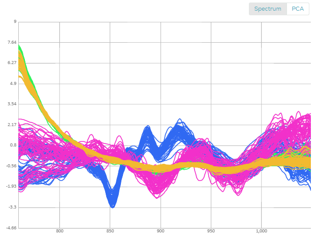
Looking at the spectra, only three are observable.

Using the PCA view, each spectrum is visualized as a point in 3D space (you can rotate the view to better see the difference between types), you can clearly see the four different medicines, the blue and purple are well separated, while the green and orange are somewhat overlapping.

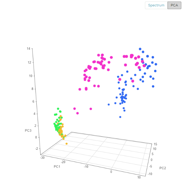
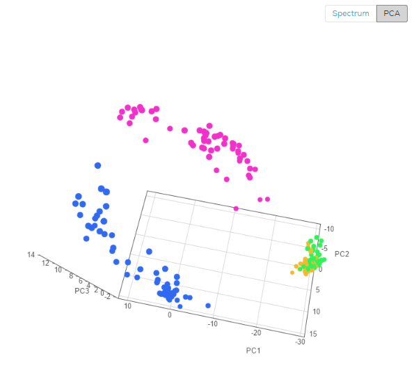
From the PCA view, one can project that a classification model on this data will work well  on the blue and purple, but will have some difficulty discerning green from orange. The next figure shows the expected performance of the classification model (AKA “confusion matrix”)

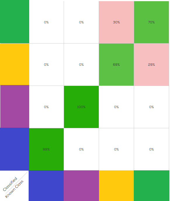
As expected, two medicines (blue and purple) are easily distinguished, and two (green and orange) have some confusion between them.

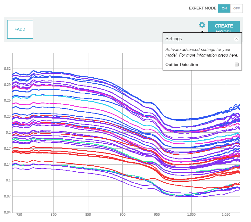
Once you have created a model you are satisfied with, you should test it on data other than the data collection used to create it. This will ensure your model works on other scans as well, and will give you more confidence regarding its robustness.
To test your model’s performance, simply click test model and select one of the other collections in your account and click test. The model will analyze each scan in the test collection, and the results will be downloaded as a text file to your computer so you can do whatever research you want on it (for example, finding the correlation between high errors and one of the attributes, estimating the performance of the outlier detection algorithm, etc.)

Latent variables can be regarded as the real information hiding in the spectra. Too many latent variables can result in an over-fitted model that will not work well on new samples.
When models are created, an optimization process decides how many latent variables will be used in the model. The default range of latent variables is 1-5 (the maximal number of LVs is limited to 20% of the number of samples).
Using the expert mode, you can choose which number of LVs to use in the optimization process by writing a new range using ‘-‘ or discrete values separated by ‘,’.

For example, if you create a simple model for mixtures of material A and material B, one LV for each material should be enough to capture the information hidden in the spectrum.

To import and export meta-data, open your target data collection and select the Samples tab.

You will see Import Data and Export Data buttons in the right hand corner.

Export Meta-Data

To export meta-data, click Export Data to download the data to a CSV file. Save the file to your computer.

Import Meta-Data

1. To upload a CSV file with meta-data of your samples (instead of doing it in the web page or during scanning), click Import Data.

Note: You will need a unique identifier per sample in both cloud and CSV file.

2. Click Choose File and select the CSV file to upload.

3. Click Next.

4. Mark the column/s of the unique sample identifier/s to be used as reference values from your file and click Next.

5. Link the attributes you want to import values from your spreadsheet,

(this is done automatically when there is a full match between column header and attribute name) and click Import.

Your meta-data will be automatically imported.

6. Click Done to complete the import and load your collection scans.

Merge Collections

Data collections were previously limited by size restrictions. This resulted in large collections being divided into smaller segments.

It is now possible to merge two collections into one single collection using the +Merge Collections tool

1. Click +Merge Collections

2. Select two collections and enter a new collection name and description

3. Click Merge. The new collection will be added to the main collections page

When you create a classification model, scan responses are related to one of the classes in the data collection. For example, if you scan only hand and desk when creating a model, when testing the model you will always get one of these classes, even if you scan something completely different (for example, orange).

The Outlier Detection feature will produce an additional scan response of ‘null’ for unrecognized materials.

Outlier Detection

If you activate the Outlier Detection mode before you create a model, when testing your model on unrecognized material the response will be “null”.

To activate Outlier Detection mode:

• Set the expert mode to On (expert mode is set as off by default)
• Click the cog wheel
• In Settings, check the Outlier Detection checkbox

What is a Model?

In SCiO, Models are the mathematical algorithms that transform data collections into data processing engines.

Models are built from data collections, which are groups of scanned samples. Samples are the collection of spectra and meta-data of sample materials.

Within the SDK, you’ll be involved in the process of SCiO Model Creation and SCiO Mobile Application building. This section of the online guide explains the modeling process, while the Mobile APIs for Android and iOS explain the application building process.

Reminder: you’ll need at least one working model before you can build a SCiO mobile application. (You can think of models as the processing brain behind each application)

The SCiO Model workflow includes the following basic steps: Model Preparation, Data Collection Definition, Data Collection Formation, Model Creation and Tweaking, Model Evaluation and Testing.

Once models are tested with good performance, SCiO mobile apps based on those models can be created.

Both individual scans, and whole samples can be deleted from SCiO Lab and from SCiO Lab Mobile.

As Scans are the building blocks of samples, they are accessed via the Samples tab in both applications.

To delete a scan from either SCiO Lab or SCiO Lab Mobile, select the Data Collection where the sample scan you want to delete exists.

1. From within the Data Collection that contains the Sample you wish to delete, select the Samples tab.
2. Select the Sample that contains the scan you want to delete from the list.
3. Select the scan you want to delete and click Delete Scan.

Sample tab view, Scan view mode

Scans can also be deleted from the Spectrum tab view. To delete from the Spectrum tab, navigate to the Sample that contains the scan you want to delete from the Spectrum Tab. Select the scan to delete from the graph view and click on its spectra. A new window will open with information about the scan and will fade the other scans from the graph view. Select More and the delete scan option will display as shown below. Delete the scan.

Spectrum tab view

Spectrum tab view, Scan data mode

To delete a Sample from SCiO Lab Mobile:

1. Tap the Data Collection with the Sample that contains the Scan you wish to delete.
2. Tap the Sample that contains the Scan you wish to delete.
3. Tap the Scan to be deleted in the list of Scans for that Sample. Delete the Scan using the trash icon on the bottom of the screen.

In addition to the scanning instructions as shown above, here are some of the best practice tips and tricks from other SCiO users in the field.

Create a Scan

Scans are the building blocks of Samples, from which we create a Data Collection, and from there build models. So in order to create a new scan, a data collection has to exist within your SCiO Lab collection into which to scan. Samples are therefore created within the Data Collection you choose when you take your first scan.

To create a scan in the SDK:

1. From SCiO Lab mobile, tap the data collection you want to scan into.
2. Tap NEW SAMPLE.
3. Complete the attributes of the sample you intend to scan. Don’t forget the photo!
4. Tap NEXT.
5. Calibrate if needed.
6. Position your Sample and your SCiO and tap SCAN.
7. Scan the sample from slightly different angles up to 3 times.
8. When finished, tap DONE.

Your scan(s) are now saved and a new sample has been created.  To access the scans, select the sample and choose any one of the scans you created from the scan list. To add further scans to a sample, tap the  + button in the bottom right corner.